


课程
Lab 08 实验报告
Lab 08 实验报告
实验题目:用线性核与高斯核训练支持向量机
计算机与信息工程学院实验报告
实验题目
用线性核与高斯核训练支持向量机
实验目的
掌握支持向量机的原理及应用
实验环境
Anaconda/Jupyter notebook
实验内容
(实验具体要求)
一、已经给定部分代码,补充完整的代码,需要补充代码的地方已经用红色字体标注,包括:
- #补充构建SVM模型及训练代码
- #补充预测代码
- #补充得到支持向量代码 二、将补充完整的代码提交,并提交实验结果;(也可以自己重写这部分的代码提交)
data_file_watermelon_3a = "watermelon_3a.csv"
import pandas as pd
import numpy as np
import matplotlib.pyplot as plt
df = pd.read_csv(data_file_watermelon_3a, header=None, )
df.columns = ['id', 'density', 'sugar_content', 'label']
df.set_index(['id'])
X = df[['density', 'sugar_content']].values
y = df['label'].values
########## SVM training and comparison
# based on linear kernel as well as gaussian kernel
from sklearn import svm
for fig_num, kernel in enumerate(('linear', 'rbf')):
#补充构建SVM模型及训练代码
#给定新的样本X_test,预测其标签
X_test = [[0.719,0.103]]
#补充预测代码
#补充得到支持向量代码
##### draw decision zone
plt.figure(fig_num)
plt.clf()
# plot point and mark out support vectors
plt.scatter( X[:,0], X[:,1], edgecolors='k', c=y, cmap=plt.cm.Paired, zorder=10)
plt.scatter(sv[:,0], sv[:,1], edgecolors='k', facecolors='none', s=80, linewidths=2, zorder=10)
# plot the decision boundary and decision zone into a color plot
x_min, x_max = X[:, 0].min() - 0.2, X[:, 0].max() + 0.2
y_min, y_max = X[:, 1].min() - 0.2, X[:, 1].max() + 0.2
XX, YY = np.meshgrid(np.arange(x_min, x_max, 0.02), np.arange(y_min, y_max, 0.02))
Z = svc.decision_function(np.c_[XX.ravel(), YY.ravel()])
Z = Z.reshape(XX.shape)
plt.pcolormesh(XX, YY, Z>0, cmap=plt.cm.Paired)
plt.contour(XX, YY, Z, colors=['k', 'k', 'k'], linestyles=['--', '-', '--'], levels=[-.5, 0, .5])
plt.title(kernel)
plt.axis('tight')
plt.show()
实验步骤
(代码截屏插入文档,清晰展示出你做的工作,得出的结果,图文并茂,让人一目了然)
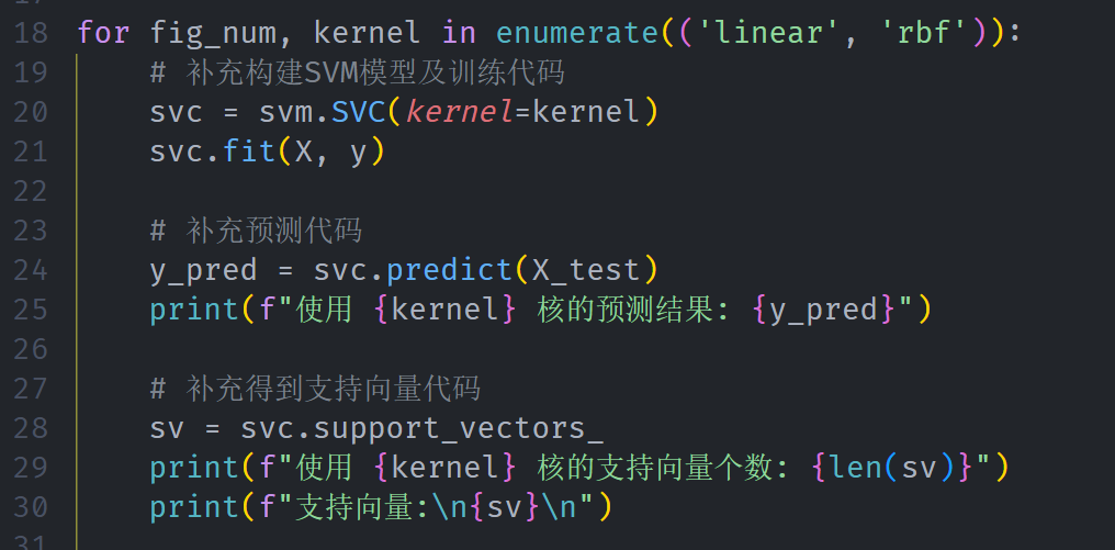
补充的代码如图
实验数据记录: (如果是已经给出的数据可以不写)
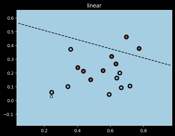
使用 linear 核的预测结果: [0]
使用 linear 核的支持向量个数: 16
支持向量
[[0.666 0.091]
[0.245 0.057]
[0.343 0.099]
[0.639 0.161]
[0.657 0.198]
[0.36 0.37 ]
[0.593 0.042]
[0.719 0.103]
[0.697 0.46 ]
[0.774 0.376]
[0.634 0.264]
[0.608 0.318]
[0.556 0.215]
[0.403 0.237]
[0.481 0.149]
[0.437 0.211]]
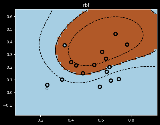
使用 rbf 核的预测结果: [0]
使用 rbf 核的支持向量个数: 16
支持向量
[[0.666 0.091]
[0.245 0.057]
[0.343 0.099]
[0.639 0.161]
[0.657 0.198]
[0.36 0.37 ]
[0.593 0.042]
[0.719 0.103]
[0.697 0.46 ]
[0.774 0.376]
[0.634 0.264]
[0.608 0.318]
[0.556 0.215]
[0.403 0.237]
[0.481 0.149]
[0.437 0.211]]
问题讨论
(实验收获,遇到的问题以及解决问题的思路路径)
使用 svm.SVC(kernel=kernel) 创建SVM分类器使用 fit(X, y) 方法进行模型训练
使用predict() 方法进行样本预测
线性核: 决策边界为直线,适用于线性可分的数据
高斯核: 可以构建非线性决策边界,适用于更复杂的数据分布
通过本次实验,验证了SVM在小样本数据集上的分类能力。线性核和高斯核虽然支持向量数量相同,但决策边界形态不同:线性核形成直线边界,高斯核形成曲线边界,能更好地拟合数据的非线性分布特征。